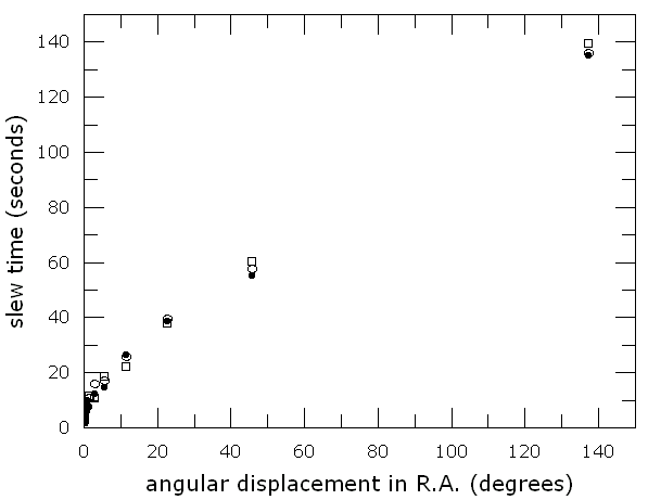
TAO - Getting Started - Step 2 (continued)

You should now have obtained data files containing tables of measured telescope slew times in right ascension and declination. If your telescope is housed in an automated dome, you would also have a data file containing a table of measured dome slew times in azimuth. Here we will assume that the right ascension, declination, and dome slew time data have been saved to files RA.txt, Dec.txt, and Az.txt, respectively, and that these files are located in directory TAO\regress. Below we describe the analysis of right ascension slew time data. The analysis of declination and azimuth slew times is completely analogous.

If you plot the data contained in RA.txt, you should obtain a well-defined relationship between angular displacement and slew time, as in the following sample plot (where three independent slew time measurements are shown for each angular displacement in right ascension; such a sample of measurements might be obtained by running script SlewTime three times in succession):

A relationship of this kind can be modeled in a simple and accurate way by a piecewise linear function, that is, a function which is linear in each of a series of intervals of the independent variable (angular displacement). The above plot shows that the relationship is essentially linear for angular displacements greater than 20 deg. In order to compute the parameters of a straight line which fits the data for displacements greater than 20 deg, one may use the least-squares program regress, which is located in the TAO\regress directory. To use this program:

Use a text editor to prepare a text file containing only those lines of RA.txt whose right ascension displacement is greater than or equal to 20 deg. For the data shown in the above plot, this file would contain these lines:
22.8557 37.9 45.7114 60.1 137.3921 139.4 22.8557 39.4 45.7114 57.7 137.3921 135.8 22.8557 38.7 45.7114 55.1 137.3921 135.0
Save this text file with a different name, e.g., TAO\regress\RA_1.txt.
Open a DOS window (Command Prompt), cd to the TAO\regress directory, and type the command
C:TAO\regress\>regress RA_1.txt

After the program executes, the regression results will have been written to file TAO\regress\RA_1_output.txt. In our example this file would contain the following results:

Regression results:

  y = A + B * x

  A =  1.87675E+01
  B =  8.58086E-01

  Coeff. of determination: R^2 =  9.98446E-01
  Standard error of B:  1.27958E-02

The high value of R² (close to unity) indicates that a good fit has been obtained (as expected from the plot), and that for angular displacements greater than 20 deg, slew time in right ascension (T, in seconds) is well approximated by the linear equation

T = 18.768 + 0.8581 x dRA,

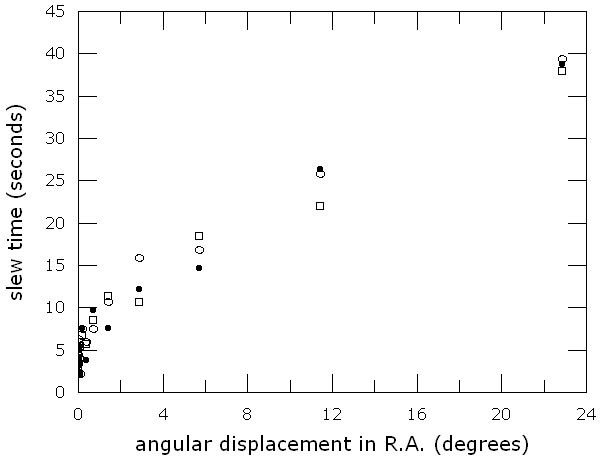
where dRA is the angular displacement in right ascension (in degrees). For angular displacements smaller than 20 deg, this relationship becomes inaccurate, so we examine more closely the lower left corner of the above plot:

We now see that the relationship is again aproximately linear for angular displacements between 1 and 20 deg, so we use regress again to fit another straight line to the corresponding data points:

T = 8.227 + 1.4541 x dRA.

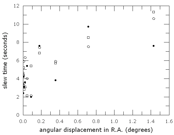
Inspecting the lower left corner of the above plot,

we see that for angular displacements smaller than 1 deg the data do not fit very well to a straight line, since the errors in the measurements of slew time become significant when compared to the slew times themselves. In any case, we use regress to fit a last straight line:

T = 3.893 + 6.36 x dRA.

After finishing the modeling of the telescope slew times in right ascension, the telescope slew times in declination and (if applicable) dome slew times in azimuth should be modeled in an analogous way.

Previous: Obtaining slew time data
Next: Preparing files containing slew time models

© 1999-2004 Paulo Holvorcem